
arviz_plots.plot_ecdf_pit#
- arviz_plots.plot_ecdf_pit(dt, *, var_names=None, filter_vars=None, group='prior_sbc', coords=None, sample_dims=None, method='envelope', envelope_prob=None, coverage=False, plot_collection=None, backend=None, labeller=None, aes_by_visuals=None, visuals=None, stats=None, **pc_kwargs)[source]#
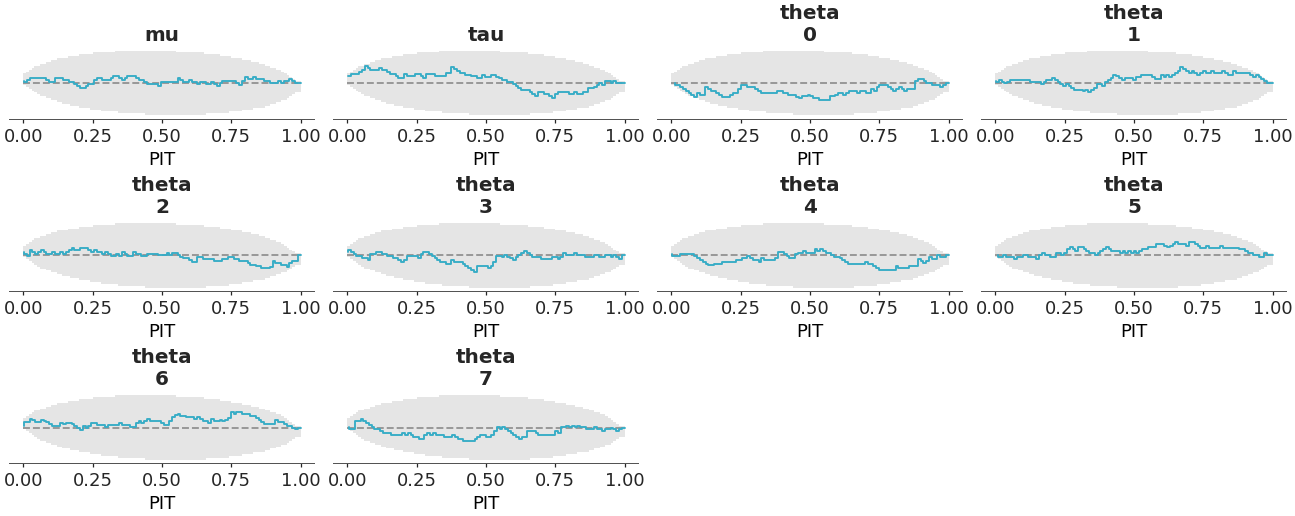
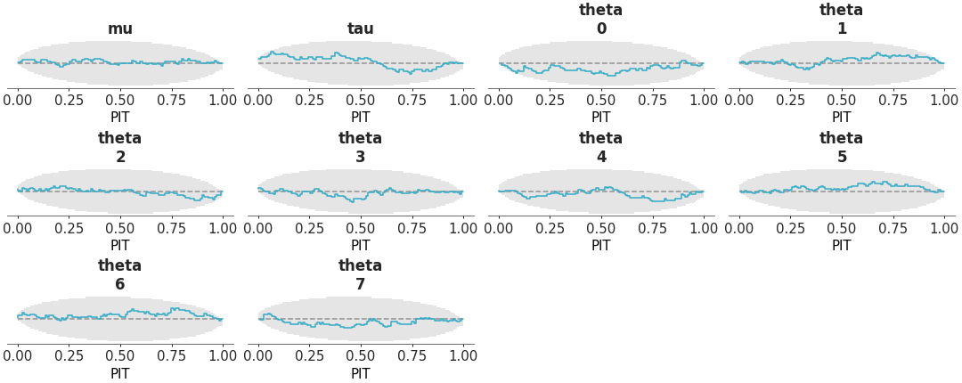
Plot Δ-ECDF.
Plots the Δ-ECDF, that is the difference between the observed ECDF and the expected CDF. It assumes the values in the DataTree have already been transformed to PIT values, as in the case of SBC analysis or values from
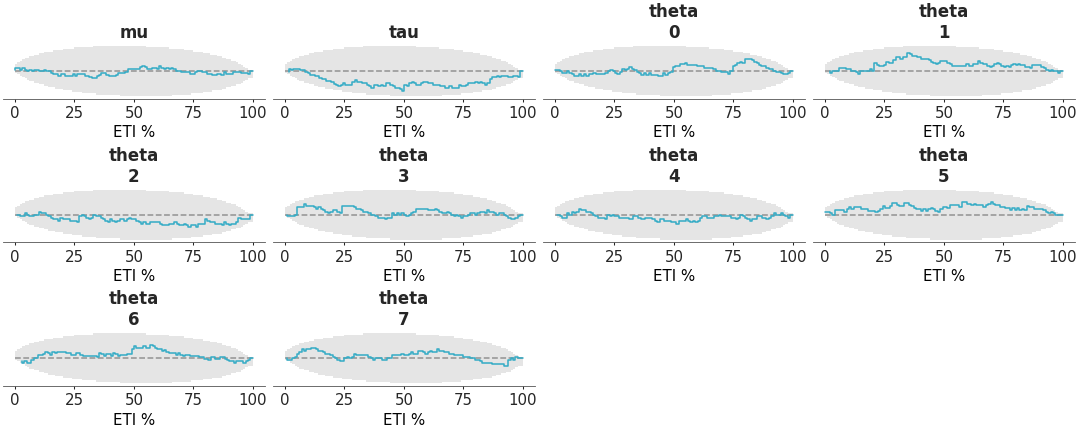
arviz_base.loo_pit.Alternatively, we can visualize the coverage of the central posterior credible intervals by setting
coverage=True. This allows us to assess whether the credible intervals includes the observed values. We can obtain the coverage of the central intervals from the PIT by replacing the PIT with two times the absolute difference between the PIT values and 0.5.For more details on how to interpret this plot, see https://arviz-devs.github.io/EABM/Chapters/Prior_posterior_predictive_checks.html#pit-ecdfs.
- Parameters:
- dt
xarray.DataTree Input data
- var_names
strorlistofstr, optional One or more variables to be plotted. Currently only one variable is supported. Prefix the variables by ~ when you want to exclude them from the plot.
- filter_vars{
None, “like”, “regex”}, optional, default=None If None (default), interpret var_names as the real variables names. If “like”, interpret var_names as substrings of the real variables names. If “regex”, interpret var_names as regular expressions on the real variables names.
- group
str, optional Which group to use. Defaults to “prior_sbc”.
- coords
dict, optional Coordinates to plot.
- sample_dims
stror sequence of hashable, optional Dimensions to reduce unless mapped to an aesthetic. Defaults to
rcParams["data.sample_dims"]- method{“pot_c”, “prit_c”, “piet_c”, “envelope”}, optional
Method to use for the uniformity test. See the “Notes” section for the full description of the different methods available.
- envelope_prob
float, optional If method is “envelope”, indicates the probability that should be contained within the envelope, otherwise indicates the probability threshold to highlight points. Defaults to
rcParams["stats.envelope_prob"].- coveragebool, optional
Defaults to
rcParams["stats.envelope_prob"].- coveragebool, optional
If True, plot the coverage of the central posterior credible intervals. Defaults to False.
- plot_collection
PlotCollection, optional - backend{“matplotlib”, “bokeh”, “plotly”}, optional
- labeller
labeller, optional - aes_by_visualsmapping of {
strsequence ofstr}, optional Mapping of visuals to aesthetics that should use their mapping in
plot_collectionwhen plotted. Valid keys are the same as forvisualsexcept for “remove_axis”- visualsmapping of {
strmapping or bool}, optional Valid keys are:
ecdf_lines -> passed to
ecdf_linecredible_interval -> passed to
fill_between_y, only when method is “envelope”ref_line -> passed to
line_xysuspicious_points -> passed to
scatter_xyp_value_text -> passed to
annotate_xyonly when method is not “envelope”xlabel -> passed to
labelled_xylabel -> passed to
labelled_ytitle -> passed to
labelled_titleremove_axis -> not passed anywhere, can only be
Falseto skip calling this function
- statsmapping, optional
Valid keys are:
ecdf_pit -> passed to
ecdf_pit. oruniformity_testdepending on the value of method.
- **pc_kwargs
Passed to
arviz_plots.PlotCollection.wrap
- dt
- Returns:
Notes
The following methods are available for testing the uniformity of the PIT values:
pot_c: Good default choice due to its good power against diverse type of local departures from the null. Preferred in almost all cases.
piet_c: Use when you specifically want to evaluate tail deviations.
prit_c: Mostly compatible with PITs computed as normalized ranks. Don’t use unless you have a specific reason to do so.
envelope: Legacy method that uses simultaneous confidence bands. It can be used when you have independent PIT values, as in the case of SBC analysis. The method is described in method described in [1]. Notice that pot_c is also valid in those cases.
The methods “pot_c”, “piet_c” and “prit_c” compute the points that contribute the most to deviations from uniformity as described in [2].
References
[1]Säilynoja et al. Graphical test for discrete uniformity and its applications in goodness-of-fit evaluation and multiple sample comparison. Statistics and Computing 32(32). (2022) https://doi.org/10.1007/s11222-022-10090-6
[2]Tasso et al. LOO-PIT predictive model checking arXiv:2603.02928 (2026).
Examples
Rank plot for the crabs hurdle-negative-binomial dataset.
>>> from arviz_plots import plot_ecdf_pit, style
>>> style.use("arviz-variat")
>>> from arviz_base import load_arviz_data
>>> dt = load_arviz_data('sbc')
>>> plot_ecdf_pit(dt, method="envelope")